6 Classification 1

Week6: 21&23/Feb/2024

This week multiple techniques for classification are learnt. The content this week focuses on (pixel-level) unsupervised and supervised classification, and overfitting. The application section includes examples of supervised classification sourced largely from literature (and also from practical).

6.1 Summary

Human is good at finding patterns in imagery while computers are not. The patterns / land cover types are useful for analysis, but it is tedious to digitize huge amount of data manually. Hence, the task is given to the computers (being more accurate and faster), extracting patterns from remote sensing data. Decision trees replicate human decisions on detecting patterns and making conclusions based on given information (expert system!). Multiple methods based on decision trees are developed to classify remote sensing image!

Image classification: Segregate pixels of a remote sensing image into groups of similar spectral character / spectral categorical classification.

6.1.1 3 types of image classification

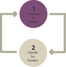
Unsupervised image classification

Unsupervised image classification: A method of categorizing data without any prior knowledge of the data [main difference with supervised classification], based solely on the inherent structure of the image itself (i.e. No ground truth examples are provided to the training algorithm / not know information on class, except the number of class).

Process: Clustering algorithm: K-means; ISODATA > number of clusters [Fewer clusters have more resembling pixels within groups. More clusters increase the variability within groups. (GISGeography 2014)] > manually assign land cover classes to each cluster

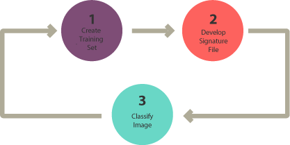
This technique addresses the issue mentioned in Week1 about the reliance on prior knowledge of the local geography when selecting training/labelling LC features. This may enhance the analysis efficiency through increasing accuracy and lowering time consumed, with the possibility of scaling up. Furthermore, patterns that are less apparent to human-eye can be detected by this technique.

The output may be harder to interpret, requiring further analysis to understand the classes. In this case, the involvement of human knowledge (not necessarily prior knowledge) would be needed to ensure the accuracy and usefulness of the outputs (which also depend on functions and data).

Supervised image classification

Supervised image classification: A method of categorizing data based on a training dataset of labeled examples.

Process: Select representative training samples for each land cover class > generate a signature file, storing all training samples’ spectral information > use the signature file to run a classification (through one of the classification algorithm: Maximum likelihood (normal distribution/parametric); Density slicing; Nearest neighbor; Minimum-distance; Principal components; Support vector machine (SVM); CART; RF; Iso cluster; Neural network) > pixel assignment > accuracy assessment

CART: a tree
RF: merging many trees, trained with bagging methods (to create a combination of learning models which improves the overall result)
SVM: optimal multi-dimensional decision hyperplane boundary that divides the dataset (test all possibilities of C and Gamma > compare with testing data > choose the combination with best accuracy)

It tends to produce highly accurate results since the training data is given by human. And it is easier to interpret to the same reason. Plus, this technique is powerful given its wide application to different data and project purposes.

As mentioned, the outcomes can be limited to the labelled classes, so it is harder to apply the same model to wider coverage / different locations where the LULC is different. Contrary to unsupervised one, this method cannot detect patterns that are not visible to human-eye / knowledge (e.g. substances under water..). Hence, more attention to training data accuracy and comprehensiveness is required (but overall this method is powerful!).

Future development on classification techniques could focus on enhancing the accuracy and reducing the need of labeling. The deep learning techniques like CNNs could be incorporated to detect complex patterns (already being developed in some cases like the Dynamic World (Brown et al. 2022)). Ancillary data can also be integrated to the imagery, being the additional context of the locations (e.g. terrain, climate, soil…). This may reduce some concerns on the difference between places/time series making the model less applicable/reproducible.

Advancement in sensors increases the possibility of recording more data in the imagery, leading to better accuracy in classification (RedEdge band in RapidEye for example). Image fusion methods are also important to allow new data to be incorporated. Optical and radar imagery fusion may allow more information being included in one analysis.

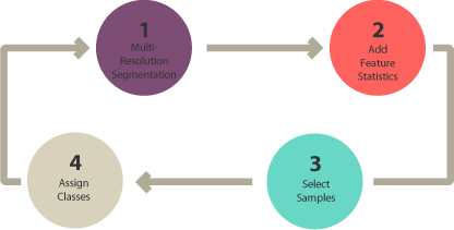
Object-based image analysis (OBIA)

Object-based image classification (more in Week7): A method integrating image segmentation with classification algorithms to group pixels together into meaningful objects/vector shapes.

6.1.2 Overfitting (of trees)

Overfitting

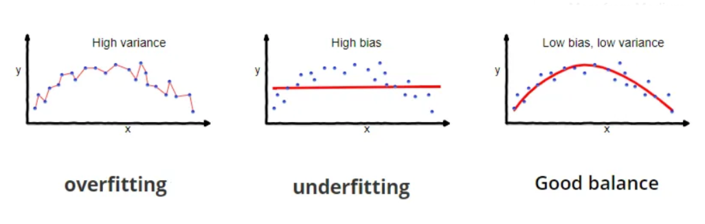
This happens when a model is trained on a limited dataset that is not representative of the full range of possible inputs, resulting in a model that performs well on the training data but poorly on new, unseen data.

It can also occur when a model is too complex and includes too many parameters, resulting in a model that is too closely tailored to the training data and unable to generalize. This is often referred to as “memorizing” the training data rather than learning from it. This will result in leaves on the decision tree having one value..

Large difference between predicted values and true value (= high bias = oversimplified model);
High variability of a model for a given point (= high variance = not generalize enough)

6.1.2.1 2 methods to balance bias and variance (regularization)

Limit the minimum number of pixels in leaves (usually 20 pixels) = top-down, easier to perform, but less mathematically sound.
Weakest link pruning with tree score (find the weakest link and delete it) = bottom-up.
- Tree score = SSR + tree penalty (alpha) * T(number of leaves)
- For all data > Use alpha=0 for all data (=full tree = SSR) > increase alpha values > find the Alpha with lowest tree score compared to the full tree when decreasing number of leaves
- Train and test split > Use the Alpha for train data > new trees > put test data in new trees > calculate SSR for test data > find the tree/alpha with the smallest SSR
- Repeat 10 times the above train and test split (using different data combinations) > find the alpha with lowest SSR across 10 repetitions
- Apply this final alpha to the whole data

Cross-validation in Week7 can also be conducted to assess the performance of the model to new data.

6.1.3 Question

(Practical) Whats the difference between .reduce(ee.Reducer.median()) and .median() ?

Tested - mostly no difference in the outputs. but the band name becomes B1_median when using reducer.median..

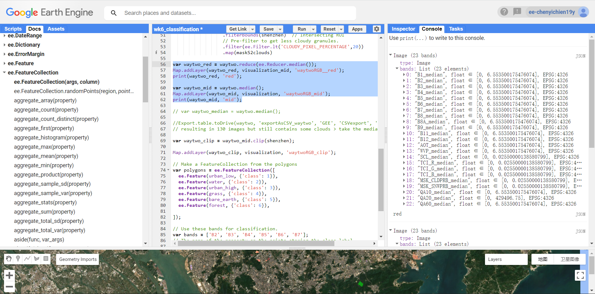
output using .reduce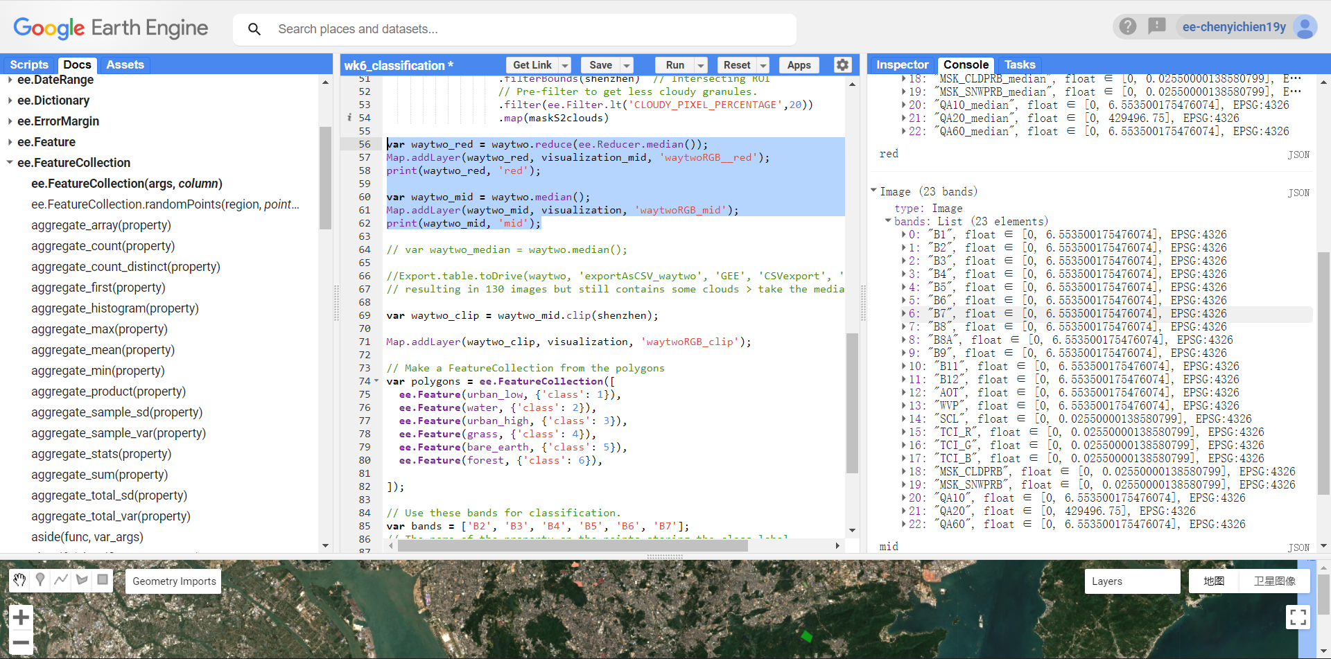

output using .median

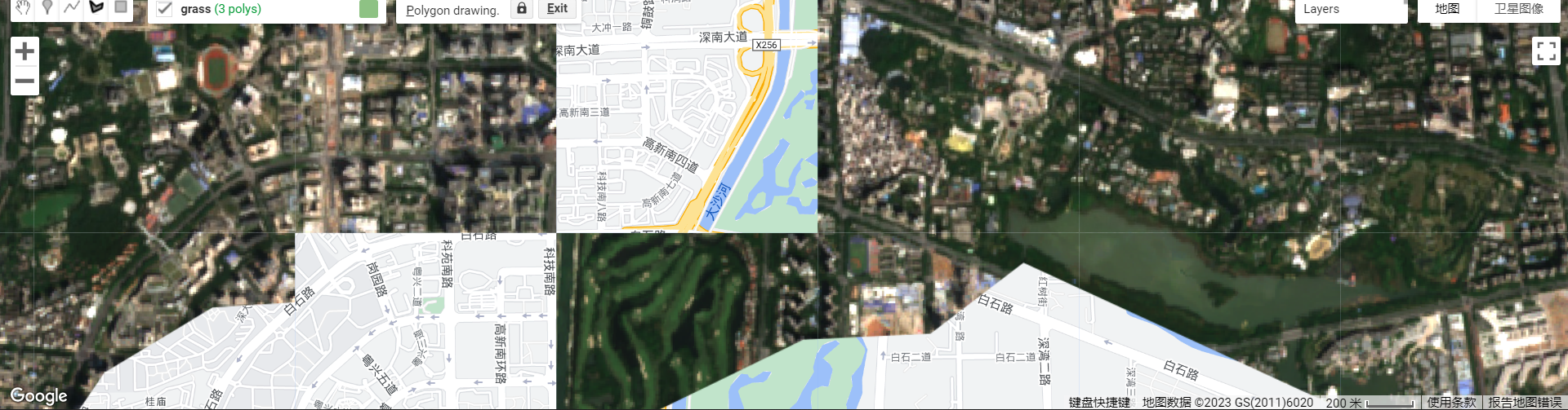
(Practical) Why the background vector map is not consistent with the remote sensing map (like the roads and buildings are not in the same position, see below snapshot)? Will this influence the data selection and accuracy (i assume other datasets may also have different consistency)?

(A: projection, but dont bother..)

(Practical) How to select high and low urban samples for training for supervised classification? (High and low as of albedo or as of density? Based on Andy’s practical workbook, it is albedo. Is this for analyzing the impact of albedo/building material on the micro-climate and earth surface temperature?)

A: Albedo - building reflectence - analysing the energy and temperature. For density - Google building data - areas of building / area of whole pixel ..

(Practical) Error occur when trying to print the training data after selecting different land cover as feature collection: FeatureCollection: Collection query aborted after accumulating over 5000 elements.

Answers online: when printing the training data, use .limit(5000) to allow printing subset of large data. (not sure if it is the right way to do, but this is the checking process afterall) (and not sure why the data is so large..)

6.2 Application

Classification of EO imagery allows extracting (and predicting) patterns/land cover from the data. This supports analysis on LULC, urban expansion, urban green space, illegal logging, forest fire, etc.

Image classification workflow: DN/reflectance of imagery > (some fieldwork / Google Earth selection of training land cover type data >) being divided based on similarities/closeness to each other using different forms of classifiers/algorithms > revealing/predicting the LULC of the Earth surface > testing accuracy > being used for further analysis / practical applications in assisting decision making.

6.2.1 CART & Random Forest

As done in the practical, the Sentinel data is classified using CART and RF. When selecting training data (selecting land cover geometries as variables), the false inference on the landuse and the inclusion of other land cover type in the geometry may add noise to the prediction, hence lowering the accuracy. Also, mentioned in the practical, when splitting the data into training and testing (for accuracy testing), the pixels of the selected geometries should be used, rather than the geometry that may add more noise to the results.

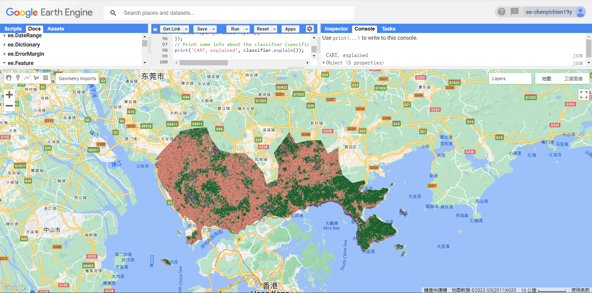
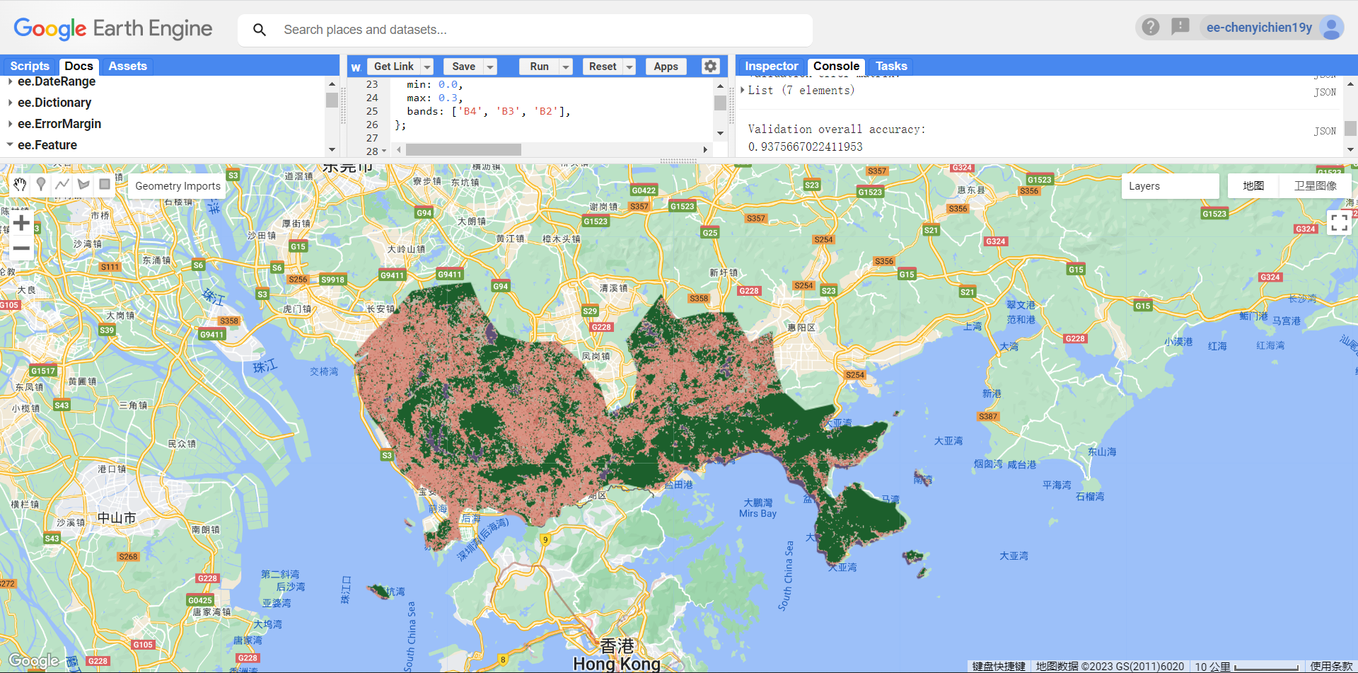
Output from practical - land cover classification using CART

Output from practical - land cover classification using RF

The accuracy is not as high as Andy’s output. For RF, the OOB error is 6%.. and the accuracy is 93%. Resubstitution accuracy is 99% (original training data vs. model output). When comparing testing data and model output, the accuracy gives 93%. > Is there any correlations between OOB accuracy and the confusion matrix? (and is it possible to add the legend to the output?)

Comparing two outputs visually, RF captures the difference in high and low urban land cover types better than CART. However, both methods produce outputs that seems like salt and pepper since they are pixel-based. Although the low urban type might exist in the forest (like meterological stations), it might not be necessary when drawing out the forest boundary. Object-based methods could be used for this purpose and for higher resolution building boundary detection for instance.

6.2.2 SVM

[Technical / methods] Study by (Ustuner, Sanli, and Dixon 2015) constructs the a classification model for agricultural landuse in Turkey using SVM method with RapidEye imargery. With fieldwork and Google Earth information on land cover types, it compares the classification accuracy with the result from Maximum Likelihood Classification (MLC) and internally among the results using different parameters (error penalty (C), gamma, bias term (r), polynomial degree (d)) and kernel types (linear, polynomial, radial basis function, sigmoid). Accuracy is assessed through kappa coefficient (comparing classified images against ground truth data). Results show that the SVM method outperforms MLC and classification accuracy is influenced by the choice of parameters (and kernels) (Ustuner, Sanli, and Dixon 2015). However, the generalization performance of kernels is influenced by the types of dataset (multi- or hyper-spectural or SAR…) so the conclusion on the best-performing kernel type is not fixed (may vary due to dataset).

[Context / application] The country’s agricultural productivity highly influence its economy. However, the data on agricultural statistics is manually collected by government employees from farmers’ declaration. The data could be unreliable (Ustuner, Sanli, and Dixon 2015) and labour-intensive, being not cost-effective for the government. Hence, methods like applying image classification on remote sensing data could provide viable, up-to-data and reliable information for sustainable crop management and planning. Before putting into practice, the sensitivity / reliability of the methods is tested through comparing between different models and within SVM using different parameters and kernels. The best combination of parameter and kernel will be used to inform decisions.

From the ground truth map, different crop types usually looks similar to human eyes while obtaining different reflectance. Hence, field works would be required to collect in-situ point data using GPS and Google Earth ancillary data could be the additional data source with experts opinions (Ustuner, Sanli, and Dixon 2015).

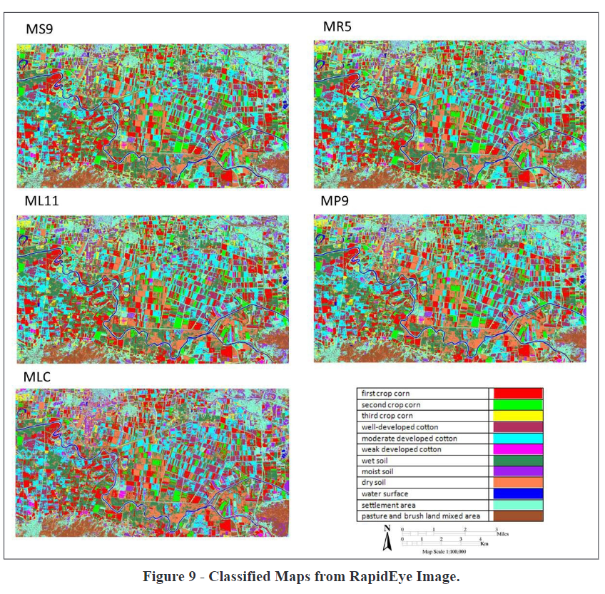
[Result / recommendation] The above output shows highest accuracy selections (compared to results from other models with different error penalty in the same kernel) of four different kernels from SVM + the result from MLC. Kappa for MS9 = 0.8209, MR5 = 0.8222, ML11 = 0.8223, MP9 = 0.8411. >> Recommendation from the authors: optimum parameters for SVM should be analyzed in detail before choosing one for best classification result.

Another study by (Pal and Mather 2005) suggests that SVM (using pair-wise comparison for multi-class) achieves higher accuracy than ML and ANN. Nevertheless, effective use depends on the values of a few user‐defined parameters. SVM in dealing with multi-class: n hyperplanes should be determined (comparing one class with the rest > may produce unclassified data, hence lowing the accuracy) or n(n-1)/2 classifiers (pair-wise comparison) (Pal and Mather 2005).

6.3 Reflection

To choose classifier, things to consider include:

Reference to literature on relevant themes might hint the direction.
Performing/comparing different classifiers might just be within several lines of code in GEE. (but.. Does the accuracy means everything? Choosing the one with highest accuracy might not be reproducible in the sense that different regions/time of year/giving new data could yield varying results?)
The choice of classifier depends on the intended outcomes and the data quality (Pragati21 2020; lanenok 2015).
1. > SVM > sparse data & binary classification & non-linear data (faster and better results, gives distance to boundary)
2. > RF > numerical and categorical features & multi-class (gives probability of belonging to class)
3. > MLC (parametric) > assuming normally distributed data (not common in LULC data > may results in lower accuracy)

Classification is valuable for urban planning mainly since its ability to identify LULC. As mentioned in previous weeks, LULC can be used to identify urban areas/growth, UHI, biodiversity and green space and flooding. It can be used in the ex-ante policy appraisal, identifying areas of improvements. Since it has information on different time series, EO data is also effective in evaluating policy outcomes / ex-post impact assessment, whereas census or other quantitative data might be constrained by the time scale and difference in sampling.