7  Classification 2

Week7: 28&2/Feb&Mar/2024

This week lecture continues to explain and evaluate other classification methods beyond pixel-level (object-based and sub-pixel) and accuracy assessment of classification outcomes. Two pre-classified models are discussed in the application section.

7.1 Summary

7.1.1 OBIA

Critique on pixel-based classification: Spatial autocorrelation (test/train) may influence the outcome of accuracy assessment (Tobler 1^st Law). If not consider SA – model would be too good / high accuracy. SA could be solved by:

1. applying distance filter/metrics or Moran’s I to the test/train data

2. or classify the image through Object-based image analysis (OBIA).

Two parameters for OBIA:

1. Distance (between centroids/seeds)

2. Homogeneity/similarity of pixels around the centroids

The output would be features of the objects (e.g. mean of the pixel values) that look like art rather than imagery. OBIA is originally applied in medical and surgery (e.g. cancer detection).

Segmentation algorithms: Multi-resolution segmentation in eCognition; The segment mean shift tool in ArcGIS > different methods to classify objects (shape; texture; spectral; geographic context; nearest neighbor)

Esp. good for high spatial resolution image by avoiding the noisiness in the outputs of pixel-based methods, more like human in processing patterns (and hence more detailed information). Because OBIA used both spectral and contextual information, it had higher accuracy compared to pixel-based methods (when comparing high and medium spatial resolution imagery) (Weih and Riggan, n.d.). > gaining popularity due to increasingly amount of high-resolution data available! More in next chapter.. Similar to supervised classification, it is also flexible in dealing with different datasets.

Segmentation can be time-consuming, computationally intensive and require some relevant knowledge. It can be biased depending on the algorithms and parameters used to define object.

7.1.2 Sub-pixel analysis

Sub-pixel analysis

The composition of pixels at a sub-pixel scale / the fraction of selected features (endmember) per pixel

Endmember

The pure spectral signatures of each land cover class

This technique may improve the accuracy of LULC classification. Due to its fine scale, detailed LC information and changes can be detected. Heterogeneity in LULC within pixel can be better classified.

Difficult to assess accuracy (due to no test/train split and accuracy depends on endmember identification) > harden. Also, the outcomes are sensitive to the spatial resolution of imagery and better outcomes depend on the high quality data input with low noise and high radiometric resolution.

Applications on pollution detection and % of vegetation

• spectrally pure ENDMEMBER selection: library (), lab, points/polygon (one point), value specification

• end-member * fraction >> unconstrained >> constrained (sum to one)

• if multiple points = MESMA

7.1.3 Accuracy Assessment

Random sampling > test/train > model output > test output > matrix

PA (producer accuracy)

\(\frac{TP}{TP+FN}\) == recall / sensitivity (correctly classified pixel vs. ground truth data)

• High PA: Low FN and High FP: e.g. predicted urban but actually other land cover type
• Error of omission = 100-PA

UA (user accuracy)

\(\frac{TP}{TP+FP}\) == precision (correctly classified pixel vs. same class pixels as classified)

• High UA: High FN and Low FP: e.g. predicted other but actually urban
• Error of commission = 100-UA

OA (overall accuracy): (TP+FP+FN+TN)

PA and UA never both good: model with Low FN and Low FP does not exist. Since data is not balanced, changes in decision threshold of classification may vary the outcomes. Increasing FP (more predicted positive) > UA worsens > FN reduces > PA improves. The matrix are related and may change together. The trade-offs between the two make the ideal situation with high PA and high UA impossible.

Hence, one of them would be more important than the other under different scenarios and the one with higher relevance to the problem should be picked when analyzing accuracy and designing the model (Wilber, n.d.):

• Recall/PA is important when we believe False Negatives are more important than False Positives (e.g. our problem of cancer detection).

• Precision/UA is important when we believe False Positives are more important than False Negatives (e.g. spam detection).

7.1.3.1 F1 score

F1 score

To solve the issue above with decision threshold, F1 score includes the information of both PA and UA in one single coefficient. \(\frac{TP}{TP+\frac{1}{2}∗(FP+FN)}\)

(Wilber, 2022)

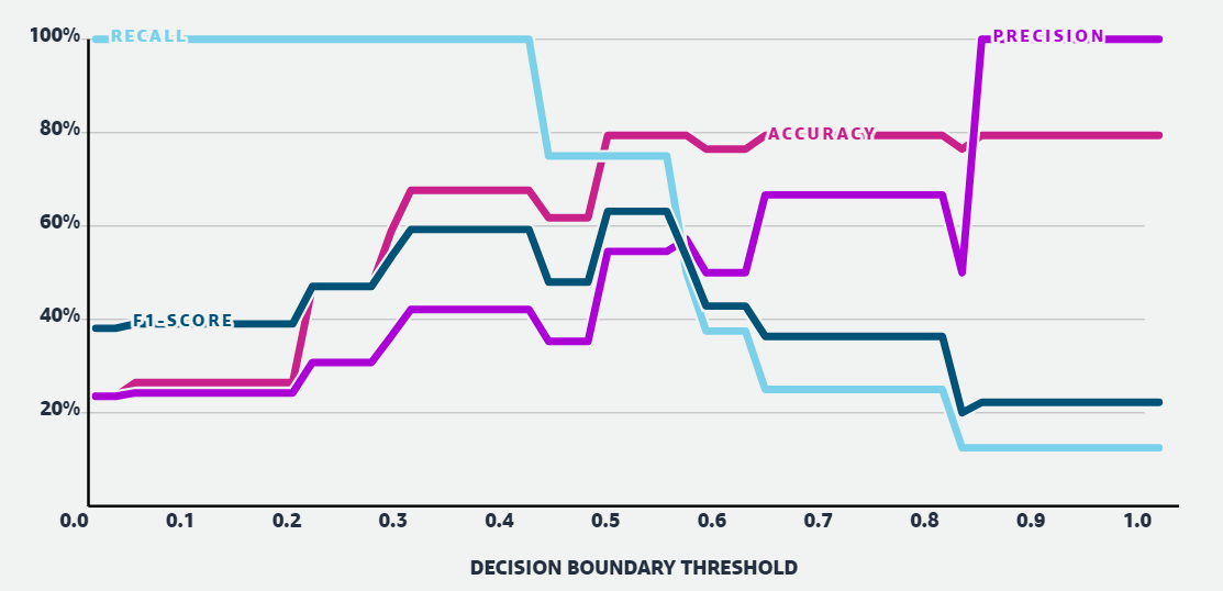
When PA and UA are similarly well-performed, the F1 and OA are also highest (when decision boundary threshold = 0.50-0.58).

Not considering TN & Assuming UA and PA equally important

Other matrix to assess accuracy: calibration, popular diagnostic tools (specificity, likelihood ratios, etc.), expectation frameworks, Receiver Operating Characteristic Curve (ROC), Area Under the Receiver Operator Characteristic Curve (AUROC) (popular for binomial model).

7.1.3.2 Kappa

Kappa coefficient

The accuracy of an image compared to the results by chance\(k=\frac{p_o−p_e}{1−p_e}\)

\(p_o\): the proportion of cases correctly classified (accuracy)

\(p_e\): expected cases correctly classified by chance

Different definitions by authors in terms of good Kappa & Different accuracy can have different ranges of kappa

7.1.3.3 Cross validation

Data-splitting: based on simple, stratified, random selection.

Repeated selection (resampling by bootstrapping): to compute the sampling variability of the accuracy metric (changing the split) (Karasiak et al. 2022)

Find the average of different scenarios to test how generalisable the model is

Randomly distributed points for testing may have spatial autocorrelation with nearby training data > influencing overestimating the accuracy / overfitting the model.

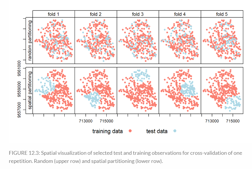
Spatial cross validation

To mitigate issue with Spatial autocorrelation in Cross validation, randomly distributed clusters of points (clustering through Moran’s I, DBSCAN, Distance metrics..) are selected for testing (Lovelace, Nowosad, and Muenchow 2019).

• reference data are also split into subsets like in cross validation but the number of subsets can vary (k-fold) (Karasiak et al. 2022).
• k-fold > random sample > > best values of C and gamma for SVM > fold >> ML3 IN R > GEE not good at data analysis but for remote sensing data

(Lovelace et al., 2019)

• mlr3 to split data for spatial CV: 3 stages: 1) task: data specification (including response and predictor variables) and the model type (such as regression or classification). 2) learner defines the specific learning algorithm that is applied to the created task. 3) resampling approach assesses the predictive performance of the model, i.e., its ability to generalize to new data. Detailed example see (Lovelace, Nowosad, and Muenchow 2019).

• Leave one out (for everything except one point) – more extreme / computationally extensive

• Selecting data for training / testing / accuracy: aim to be reproducible (same model for different years data) by choosing land that not change to much (pseudo-invariant features) / manual selection of ROI / choose same parcels/features from different years to make the model generalizable. There is no fixed rule on this.

7.2 Application

Below are some examples of pre-classified data that could be imported in GEE.

7.2.1 Dynamic world

• GEE data catalog

Process: World / region / biomes > experts / non-experts to label training pixels (5x5) > pre-processing (> TOA > rotate > band math/ratioing) > normalisation (log) > classification (CNN)

Near real time data at 10m resolution (Sentinel-2 with 2-5 days revisit)

Blobbing – since ppl/users train data + CNN (deep learning, moving window of filtering..)

7.2.2 Google open building data

• GEE data catalog

This dataset includes building info like outlines, footprints on the ground, confidence score (on if this is a building / accuracy), the centroid of the building (not having info like building typology, address, and other details beyond geometry).

50cm high-resolution

Currently constrains to Africa, South Asia and South-East Asia locations

Thoughts on applications suggested by developers:

• Population mapping: largely related to the population estimates based on building block. Estimating population based on building outline seems less convincing as the building height data is not assessed. This could be solved by combining the method of detecting building shades from satellite imagery and sample building height annotations with longitude, latitude, and elevation from the ICESat-2, ATL03 photons (Zhao et al. 2023). Hence, a 3D building data can be used to estimate population more accurately. However, the population density per building may vary spatially and over time, influenced by the building functions. Offices for instance should be omitted during prediction. The detailed land use type per building may be beyond the scope of remote sensing data. That said, population estimation for informal settlements can be valuable, which is not included in the census data.

• Humanitarian response: the location and density of settlements could be used to evaluate the risk zones and potential loss due to natural disasters, integrated with deep learning from data like past disaster events, social media, and weather reports to forecast the affected areas and consolidate early-warning system. Te detailed methods may subject to the types of disasters (flooding/earthquake/landslide/volcanic eruptions..). Corresponding interventions (e.g. relocation of hospitals and residence within the risk zones) in relation to the local demographics of vulnerable groups can be integrated to reduce risks, complying to the Sendai Framework for Disaster Risk reduction 2015-2030. Nevertheless, the LULC classifications may already achieve this goal, albeit without building outline..

• Addressing systems & Statistical indicators: the location of buildings can be used to simulate transport demands and routing, hence planning a more robust transport system.

Other possible uses of the data:

• Planning support: The space between buildings / street width could be useful for analyzing the environmental conditions in urban public realm, guiding regulations on building heights – narrow streets with high buildings should be avoided, increasing wind speed and reducing daylight penetration.

7.2.2.1 Accuracy

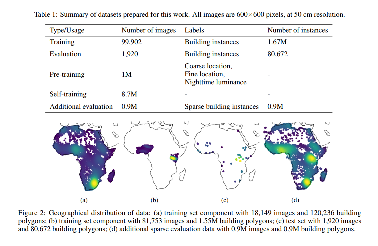
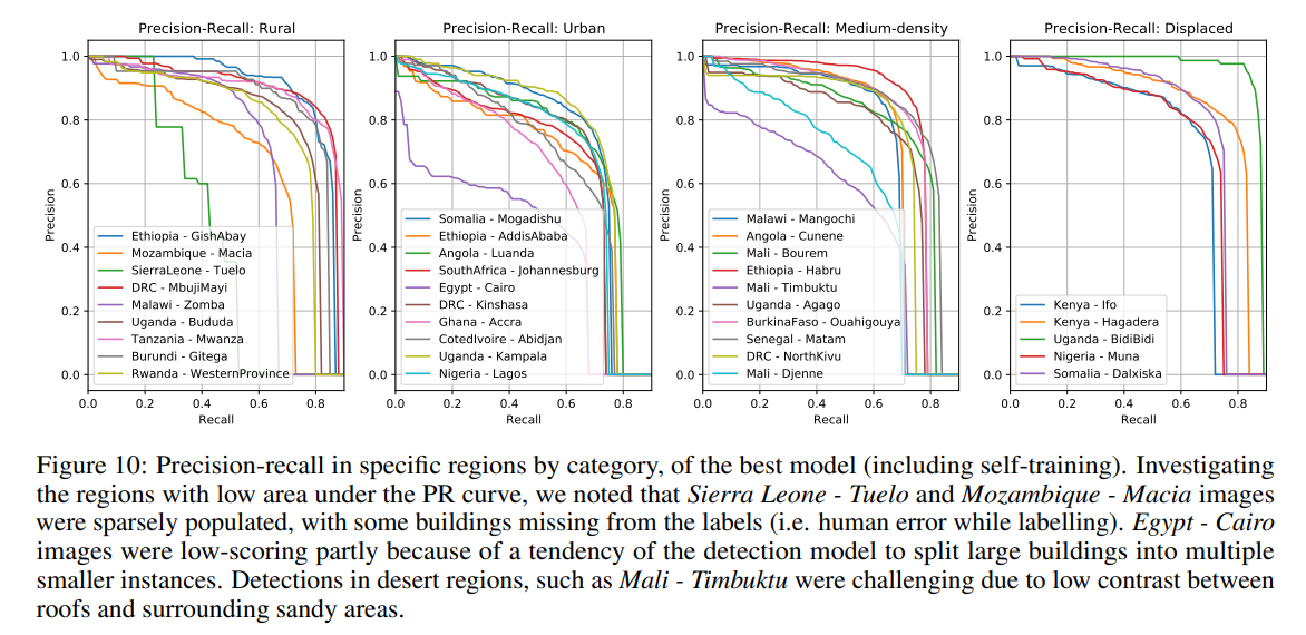
The accuracy is enhanced through the novel method using U-Net Model (mixup, self-training, distance weighting with Gaussian convolutions, and residual decoder blocks) (Sirko et al., n.d.). For randomly selected test data (Figure2c), the areas with potential bias are omitted, including those with vast rural land and empty area (.ibid).

(Sirko et al, 2021)

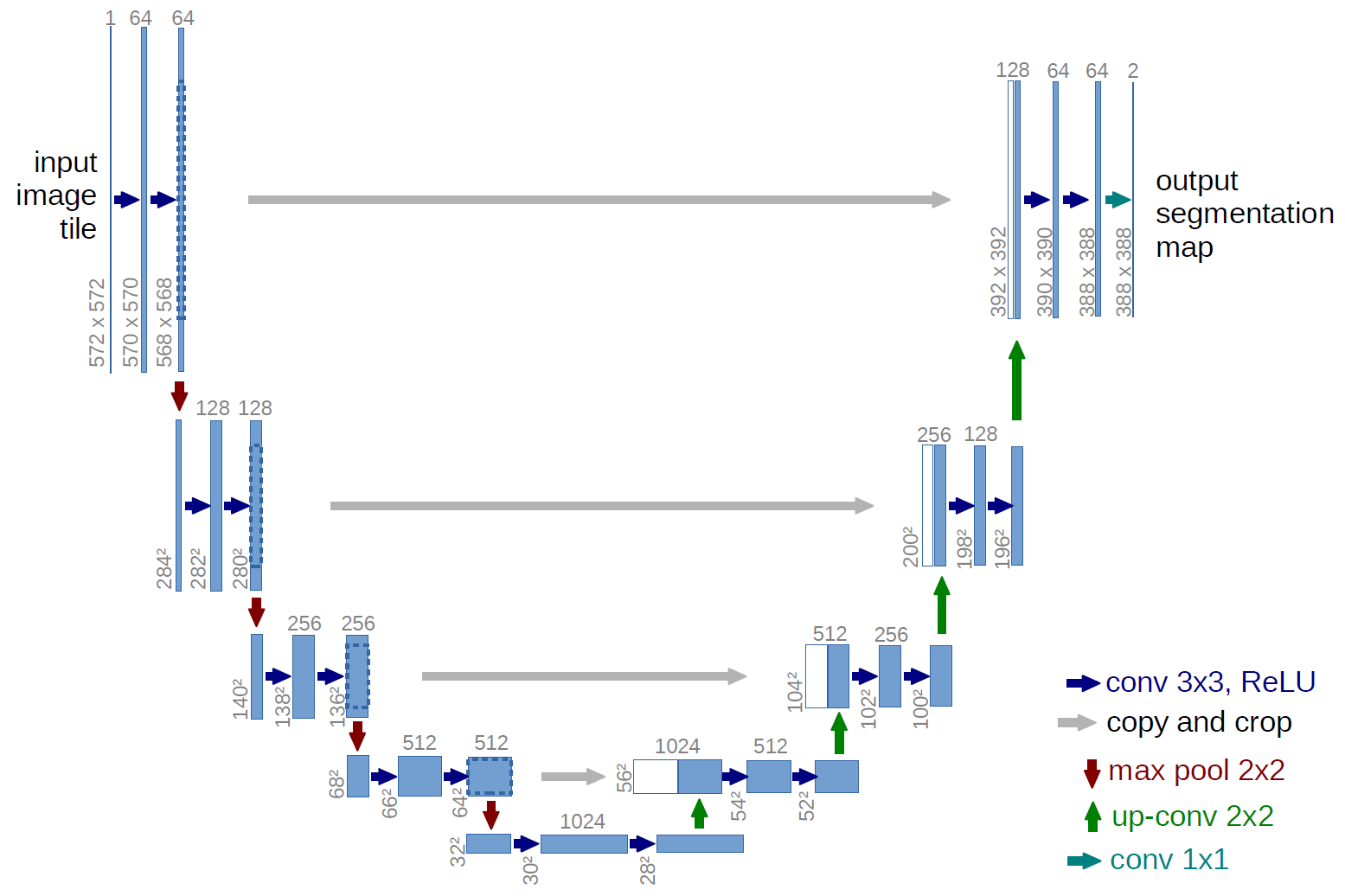
U-Net Model originates from biomed image semantic segmentation (Ronneberger, Fischer, and Brox 2015; Li et al. 2021), having wide range of applications in different fields, outperforming the original sliding-window convolutional network.

U-Net Architecture (Ronneberger, Fischer and Brox, 2015)

The performance of open building data can be accessed from the confidence score. However, there is difference in the performance spatially. Some areas like single building in rural area and dessert terrain can have lower accuracy (Sirko et al., n.d.). In urban areas, large buildings may be split into smaller ones, with most cases seen in Egypt - Cairo (ibid.).

(Sirko et al, 2021)

7.3 Reflection

Accuracy of LULC classification is essential for analysis. Various factors may contribute to the accuracy of model outputs. The quality of ground truth data could be improved in future development through novel channels like Dynamic World deploying crowdsourcing knowledge. High-resolution information from unmanned aerial vehicles can be used as the source.

In terms of urban planning, the information on Earth’s surface is sometimes not enough. A site with LULC being classified as urban land does not help the planners to identify which specific land use it is (although nightlight data can be used to imply some retail/high streets). Although land use maps are available from OSM or Digimap for example, those maps/data are usually incompatible with GEE or other processing software. Hence, it would be more powerful if the EO data can obtain land use information like offices, housing, etc. This may be done by scrapping/accessing planning application documents, or using crowdsourcing data and Google Maps, or analyzing the time people use those buildings. (Nevertheless, this might be too complicated and not worth the effort, compared to adding EO data (like air pollution) to the land use map as different layers, which already exist). Planners could use this information to refine planning guidance and masterplan. For instance, areas suffering from UHI could be assessed by land use to give further interventions. Residential land may require measures on passive cooling esp. at night while offices/retail areas may focus on daytime energy-saving appliances and effective sharing/co-working space. Public space and the private realm can also be identified with land use information, hence differentiating the interventions that could be taken.

Karasiak, N., J.-F. Dejoux, C. Monteil, and D. Sheeren. 2022. “Spatial Dependence Between Training and Test Sets: Another Pitfall of Classification Accuracy Assessment in Remote Sensing.” Machine Learning 111 (7): 2715–40. https://doi.org/10.1007/s10994-021-05972-1.

Li, Meng-Yi, Ding-Ju Zhu, Wen Xu, Yu-Jie Lin, Kai-Leung Yung, and Andrew W. H. Ip. 2021. “Application of U-Net with Global Convolution Network Module in Computer-Aided Tongue Diagnosis.” Journal of Healthcare Engineering 2021 (November): e5853128. https://doi.org/10.1155/2021/5853128.

Lovelace, Robin, Jakub Nowosad, and Jannes Muenchow. 2019. Chapter 12 Statistical Learning | Geocomputation with R. https://r.geocompx.org/spatial-cv.html.

Ronneberger, Olaf, Philipp Fischer, and Thomas Brox. 2015. “U-Net: Convolutional Networks for Biomedical Image Segmentation.” In, edited by Nassir Navab, Joachim Hornegger, William M. Wells, and Alejandro F. Frangi, 9351:234–41. Cham: Springer International Publishing. http://link.springer.com/10.1007/978-3-319-24574-4_28.

Sirko, Wojciech, Sergii Kashubin, Marvin Ritter, Abigail Annkah, Yasser Salah Eddine Bouchareb, Yann Dauphin, Daniel Keysers, Maxim Neumann, Moustapha Cisse, and John Quinn. n.d. “Continental-Scale Building Detection from High Resolution Satellite Imagery.”

Weih, Robert C, and Norman D Riggan. n.d. “OBJECT-BASED CLASSIFICATION VS. PIXEL-BASED CLASSIFICATION: COMPARITIVE IMPORTANCE OF MULTI-RESOLUTION IMAGERY.”

Wilber, Jared. n.d. “Precision and Recall.” https://mlu-explain.github.io/precision-recall/.

Zhao, Yi, Bin Wu, Qiaoxuan Li, Lei Yang, Hongchao Fan, Jianping Wu, and Bailang Yu. 2023. “Combining ICESat-2 Photons and Google Earth Satellite Images for Building Height Extraction.” International Journal of Applied Earth Observation and Geoinformation 117 (March): 103213. https://doi.org/10.1016/j.jag.2023.103213.